5_Vectors and Matrices
In this lesson we review the mathematical foundations that make geometric transformations possible in computer graphics: vectors and matrices.
Introduction
In computer graphics, we often need to do movements such as translation, scaling, and rotation. These calculations are called transformations because they change the coordinates of vertices. Especially in animated or interactive computer graphics applications, transformations are very common and they rely on the mathematical concepts of vectors and matrices.
In this lesson, we will briefly review scalars, points, and vectors before we dive into matrices.
Scalars, Points, and Vectors
Scalars
A scalar is a number representing a single quantity, such as length. Here, $c$ is a fixed value:
\(x = c\)
Points
A point is a single location in a coordinate system.
\(P=(x,y)\)
Vectors
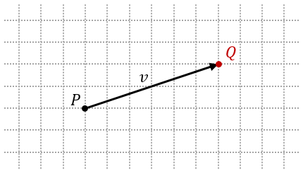
A vector represents displacement (the amount of change in a coordinate) and is drawn on graphs with an arrow.
The arrow begins at at the initial point, called the tail, and ends at the terminal point, called the head.
The distance between the tail and the head is the length or magnitude of the vector.
When the vector’s initial point is at the origin of the coordinate system, it is in standard position. When a vector $v$ is in standard position, its components describe the coordinates of its terminal point.
In the vector definition above, $dx$ is the change in the $x$-coordinate and $dy$ is the change in the $y$-coordinate.
Geometric Operations
Vector addition
Vector addition happens when we place the tail of one vector at the head of another vector. Mathematically, the addition of two vectors $v$ and $w$ can be described with the resulting vector $u$:
\[\begin{aligned} v + w & = u \\ & = \langle v_1,v_2 \rangle + \langle w_1,w_2 \rangle \\ & = \langle v_1+w_1,v_2+w_2 \rangle \\ & = \langle u_1,u_2 \rangle \end{aligned}\]If we draw the vectors head-to-tail, the resulting vector $u$ will have the initial point of vector $v$ and terminal point of vector $w$.

Vector/Point Addition
When we add vector $v$ to point $P$, we arrive at another point $Q$. This can be described mathematically: \(\begin{aligned} P+v & = Q \\ & =(P_1,P_2)+ \langle v_1,v_2 \rangle \\ & =(P_1+v_1,P_2+v_2) \\ & =(Q_1,Q_2) \end{aligned}\) The result represents translating from point $P$ to point $Q$. This means $P$ is the initial point of $v$ and $Q$ is the terminal point of $v$.
Point Subtraction
If $P+v=Q$ describes the translation from $P$ to $Q$, then we can calculate the vector $v$ connecting $P$ and $Q$ with $Q-P=v$. In other words, the displacement vector $v$ is the distance between points $P$ and $Q$, or the difference between the coordinates of $P$ and $Q$:
\[\begin{aligned} v & = Q - P \\ & = (Q_1,Q_2)-(P_1,P_2) \\ & = \langle Q_1-P_1,Q_2-P_2\rangle \\ & = \langle v_1,v_2 \rangle \end{aligned}\]Scalar Multiplication
We can scale a vector’s length, or magnitude, by multiplying it with a scalar value $c$. When the value of $c$ is negative, it effectively reverses the direction of the vector.
\[c \cdot v=c\cdot\langle v_1,v_2 \rangle = \langle c \cdot v_1,c \cdot v_2 \rangle\]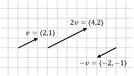
Standard Basis
The properties of vector addition and scalar multiplication allow us to express vectors in terms of a standard basis of two vectors $i= \langle 1,0 \rangle$ and $j= \langle 0,1 \rangle$. The standard basis expresses a vector $v$ as the addition of the $i$ and $j$ vectors scaled to the respective $x$-coordinate and $y$-coordinate: \(\begin{aligned} v & = \langle x,y \rangle \\ & = \langle x+0,0+y \rangle \\ & = \langle x,0 \rangle + \langle 0,y \rangle \\ & = x \cdot\langle 1,0 \rangle + y \cdot\langle 0,1 \rangle \\ & = x \cdot i+y \cdot j \end{aligned}\)
This will become very useful later when we want to represent transformations with linear functions.
Linear Transformations and Matrices
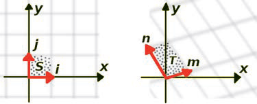
A linear transformation is a mathematical operation that converts coordinates from one vector space to another while maintaining relative structure. For example, in the figure below, the image on the left shows an object S with coordinates in terms of vectors i and j in its own vector space. When rendering the same object from a certain camera angle in a 3D scene, it may appear as the image on the right, which shows T with coordinate vectors m and n in the screen’s vector space.
We use special functions for calculating transformations based on whether they operate on a point, a vector, or multiple vectors (a matrix).
Point, Vector, and Matrix Transformations
When moving 3D objects around a scene or adjusting the camera, we need to transform their vectors so they can render at the correct position, scale, pitch, rotation, etc. Transformations are represented mathematically as vector functions, or functions that take vectors as inputs and give vectors as outputs. They can be written in three different ways depending on what the input vector represents:
Point transformation
Here, the input and output is the terminal point of a vector in standard position.
\(F \left( \left( p_1,p_2 \right) \right) = \left( q_1,q_2 \right)\)
Vector transformation
\(F \left( \langle v_1,v_2 \rangle\right) = \langle w_1,w_2 \rangle\)
Matrix transformation
Matrices are regularly used to compute the vertices of multi-dimensional objects.
\(F \left(
\begin{bmatrix}
v_1 \\
v_2
\end{bmatrix}
\right) =
\begin{bmatrix}
w_1 \\
w_2
\end{bmatrix}\)
Standard Vector Functions
Standard vector functions are simple examples of vector functions. These include the zero function, which converts any vector to the zero vector, and the identity function, which always returns the input vector without change:
Zero Function \(F\left( \langle v_1,v_2 \rangle \right) = \langle v_1 \cdot 0,v_2 \cdot 0 \rangle = \langle 0,0 \rangle\)
Identity Function \(F\left( \langle v_1,v_2 \rangle \right) = \langle v_1 \cdot 1,v_2 \cdot 1 \rangle = \langle v_1,v_2 \rangle\)
Linear Functions
Vector functions are essential to calculating transformations. They are formally known as linear functions. When we use them to describe transformations, they become linear transformations.
Linear transformations are very useful in CG due to the properties of vector functions for scalar multiplication and vector addition.
Scalar multiplication of vector functions
\(F(c \cdot v) = c \cdot F(v)\)
Vector addition of vector functions
\(F(v+w) = F(v) + F(w)\)
And we can even combine scalar multiplication with vector addition: \(F(c \cdot v + d \cdot w) = c \cdot F(v) + d \cdot F(w)\)
This shows that we can simplify any complicated linear function by first the applying the function to the vectors individually and then combining the results. A common shortcut for calculating linear transformations is to rewrite them in terms of the standard basis vectors $i=\langle 1,0 \rangle$ and $j=\langle 0,1 \rangle$. This way, we don’t actually need to know how the function calculates any given transformation. We only need to know the results of transforming the standard basis vectors.
Given the standard basis of a vector $v$, \(v = \langle x,y \rangle = x \cdot i+y \cdot j\)
and properties of linear functions, \(F(c \cdot v+d \cdot w) = c \cdot F(v)+d \cdot F(w)\)
we can find $F(v)$ for any vector $v=\langle x,y \rangle$ as: \(\begin{aligned} F(v) &= F\left( \langle x,y \rangle \right)\\ &= F(x \cdot i+y \cdot j) \\ &= x \cdot F(i)+y \cdot F(j) \end{aligned}\)
Now it is possible to transform any vector from one space to another when we know the results of the linear function for the standard vectors, as expressed by $F(i)$ and $F(j)$.
Here is an example: given $F(i)= \langle 2,1 \rangle$ and $F(j)= \langle -1,3 \rangle$, we can find $F(v)$ where $v= \langle 4,5 \rangle$, \(\begin{aligned} F( \langle 4,5 \rangle ) &= F( \langle 4,0 \rangle + \langle 0,5 \rangle) \\ &=F( \langle 4,0 \rangle ) + F( \langle 0,5 \rangle ) \\ &=F(4 \cdot \langle 1,0 \rangle) + F(5 \cdot \langle 0,1 \rangle) \\ &=4 \cdot F( \langle 1,0 \rangle ) + 5 \cdot F( \langle 0,1 \rangle ) \\ &=4 \cdot F(i)+ 5 \cdot F(j) \\ &=4 \cdot \langle 2,1 \rangle + 5 \cdot \langle -1,3 \rangle \\ &=\langle 8,4 \rangle + \langle -5,15 \rangle \\ &=\langle 3,19 \rangle \end{aligned}\)
Matrices
Calculating linear transformations can be pretty simple if we represent the values of $F(i)$ and $F(j)$ with variables to find a pattern. Let’s say $F(i) = \langle a,c \rangle$ and $F(j) = \langle b,d \rangle$. Then, \(\begin{aligned} F( \langle x,y \rangle ) &= x \cdot F(i)+y \cdot F(j) \\ &= x \cdot \langle a,c \rangle + y \cdot \langle b,d \rangle \\ &= \langle a \cdot x,c \cdot x \rangle + \langle b \cdot y,d \cdot y \rangle \\ &= \langle a \cdot x+b \cdot y,c \cdot x+d \cdot y \rangle \end{aligned}\)
Then, rewrite $F( \langle x,y \rangle) = \langle a \cdot x+b \cdot y,c \cdot x+d \cdot y \rangle$ with the matrix notation from above and we see all the scalar values can be expressed as a matrix by themselves: \(\begin{aligned} F \left( \begin{bmatrix} x \\ y \end{bmatrix} \right) &= \begin{bmatrix} a \cdot x+b \cdot y \\ c \cdot x+d \cdot y \end{bmatrix} \\ &= \begin{bmatrix} a & b \\ c & d \end{bmatrix} \cdot \begin{bmatrix} x \\ y \end{bmatrix} \end{aligned}\)
In other words, the transformation function $F$ can be expressed as $F(v)=A \cdot v$ where $A$ is the transformation matrix applied to vector $v$.
For example, let’s consider again the transformation from above where $F(i)= \langle 2,1 \rangle$ and $F(j)= \langle -1,3 \rangle$, then calculate $F(\langle 4,5 \rangle)$: \(\begin{aligned} F\left( \begin{bmatrix} 4 \\ 5 \end{bmatrix} \right) &= \begin{bmatrix} 2 & -1 \\ 1 & 3 \end{bmatrix} \cdot \begin{bmatrix} 4 \\ 5 \end{bmatrix} \\ &= \begin{bmatrix} 2 \cdot 4+-1 \cdot 5 \\ 1 \cdot 4+ 3\cdot 5 \end{bmatrix} \\ &= \begin{bmatrix} 8 + -5 \\ 4 + 15 \end{bmatrix} \\ &= \begin{bmatrix} 3 \\ 19 \end{bmatrix} \end{aligned}\)
Using the concepts of matrix multiplication, we can find the transformation matrices of the standard vector functions from before. Here is the zero function: \(F\left( \begin{bmatrix} x \\ y \end{bmatrix} \right) = \begin{bmatrix} 0 \\ 0 \end{bmatrix} = \begin{bmatrix} 0 \cdot x+0 \cdot y \\ 0 \cdot x+0 \cdot y \end{bmatrix} = \begin{bmatrix} 0 & 0\\ 0 & 0 \end{bmatrix} \cdot \begin{bmatrix} x \\ y \end{bmatrix}\)
And here is the identity function: \(F\left( \begin{bmatrix} x \\ y \end{bmatrix} \right) = \begin{bmatrix} x \\ y \end{bmatrix} = \begin{bmatrix} 1 \cdot x+0 \cdot y \\ 0 \cdot x+1 \cdot y \end{bmatrix} = \begin{bmatrix} 1 & 0\\ 0 & 1 \end{bmatrix} \cdot \begin{bmatrix} x \\ y \end{bmatrix}\)
The matrix from the definition of the identity function is called the identity matrix which is often represented with the letter $I$ as in,
\[I=\begin{bmatrix} 1 & 0 \\ 0 & 1 \end{bmatrix}\]Now since matrices of different sizes are used for multiple dimensions beyond 2D, things quickly become messy if we continue to use $a$, $b$, $c$, etc. Instead, it is common to express matrix components with double subscripts such as $a_{mn}$ where $m$ is the row and $n$ is the column of the component $a_{mn}$. A 2x2 matrix written with this notation would be: \(A=\begin{bmatrix} a_{11} & a_{12} \\ a_{21} & a_{22} \end{bmatrix}\)
Then we can add more rows and columns by incrementing the values of $m$ and $n$ in the new components.
Matrix Composition
Rendering computer graphics from scene data often requires applying many different transformations to point coordinates. For example, we may need to scale an object, rotate it, then apply one more transformation to get its coordinates in the camera space. This could involve three (or more) linear functions—one for each transformation.
The composition of two linear functions $F$ and $G$ applied to vector $v$ describes using the result of $G(v)$ as the input for function $F$, effectively applying the functions in the order of $G$ followed by $F$. Here $H$ represents the composition and is written as, \(H(v)=F(G(v))\)
The properties of linear functions hold true for compositions of linear functions as well.
Here is scalar multiplication:
\(\begin{aligned}
H(c \cdot v)&=F(G(c \cdot v)) \\
&=F(c \cdot G(v)) \\
&=c \cdot F(G(v)) \\
&=c \cdot H(v)
\end{aligned}\)
And vector addition:
\(\begin{aligned}
H(v+w)&=F(G(v+w)) \\
&=F(G(v)+G(w)) \\
&=F(G(v))+F(G(w)) \\
&=H(v)+H(w)
\end{aligned}\)
Combining scalar multiplication and vector addition, we have:
\(\begin{aligned}
H(c \cdot v+d \cdot w) &= F(G(c \cdot v+d \cdot w)) \\
&= F(G(c \cdot v)+G(d \cdot w)) \\
&= F(c \cdot G(v)+d \cdot G(w)) \\
&= F(c \cdot G(v))+F(d \cdot G(w)) \\
&= c \cdot F(G(v))+d \cdot F(G(w)) \\
&= c \cdot H(v)+d \cdot H(w)
\end{aligned}\)
This means that we can represent any number of compositions as a single matrix which we find by simply multiplying together the matrices of each linear function!
That is, when $F(v)=A \cdot v$ and $G(v)=B \cdot v$, then $H(v)=C \cdot v$ where $C=A \cdot B$. \(H(v)=F(G(v))=A \cdot (B \cdot v)=(A \cdot B) \cdot v=C \cdot v\)
When we expand $H(v)=C \cdot v$ in terms of components we get: \(\begin{aligned} C \cdot v &= (A \cdot B) \cdot v \\ &= \left( \begin{bmatrix} a_{11} & a_{12} \\ a_{21} & a_{22} \end{bmatrix} \cdot \begin{bmatrix} b_{11} & b_{12} \\ b_{21} & b_{22} \end{bmatrix} \right) \cdot \begin{bmatrix} x \\ y \end{bmatrix} \\ &= \begin{bmatrix} (a_{11} \cdot b_{11} + a_{12} \cdot b_{21}) & (a_{11} \cdot b_{12} + a_{12} \cdot b_{22}) \\ (a_{21} \cdot b_{11} + a_{22} \cdot b_{21}) & (a_{21} \cdot b_{12} + a_{22} \cdot b_{22}) \end{bmatrix} \cdot \begin{bmatrix} x \\ y \end{bmatrix} \\ &= \begin{bmatrix} c_{11} & c_{12} \\ c_{21} & c_{22} \end{bmatrix} \cdot \begin{bmatrix} x \\ y \end{bmatrix} \end{aligned}\)
So, the composition matrix is the product of the two transformation matrices $A$ and $B$:
\(\begin{aligned}
C &= A \cdot B \\
&=\begin{bmatrix}
(a_{11} \cdot b_{11} + a_{12} \cdot b_{21}) & (a_{11} \cdot b_{12} + a_{12} \cdot b_{22}) \\
(a_{21} \cdot b_{11} + a_{22} \cdot b_{21}) & (a_{21} \cdot b_{12} + a_{22} \cdot b_{22})
\end{bmatrix} \\
&= \begin{bmatrix}
c_{11} & c_{12} \\
c_{21} & c_{22}
\end{bmatrix}\end{aligned}\)
Inverse Transformations
Representing geometric transformations as vector functions allows us to incorporate the idea of “opposite” or “reverse” transformations for any given function. For example, displacing a point by vector $\langle m,n \rangle$ has an inverse displacement of $\langle -m,-n \rangle$; rotating an object by angle $a$ has an inverse rotation of $-a$; and scaling object components by magnitude $r$ has an inverse scale of $1/r$.
When we compose a transformation function with its inverse, the output is the same as the input. That is, when $G$ is the inverse of $F$, then $F(G(v))=v$. This implies that the matrix of $F$ and the matrix of $G$ must be inverses of each other which we write as $A$ and $A^{-1}$. Just as multiplying a scalar $r$ with its inverse $1/r$ yields $1$, the composition of a matrix with its inverse is the identity matrix from before: \(F(G(v))=A \cdot A^{-1} \cdot v=I \cdot v= \begin{bmatrix} 1 & 0 \\ 0 & 1 \end{bmatrix} \cdot \begin{bmatrix} x \\ y \end{bmatrix} = \begin{bmatrix} x \\ y \end{bmatrix}\)
In terms of the matrix components, \(A \cdot A^{-1}=\begin{bmatrix} a & b \\ c & d \end{bmatrix} \cdot \begin{bmatrix} e & f \\ g & h \end{bmatrix} = \begin{bmatrix} 1 & 0 \\ 0 & 1 \end{bmatrix} = I\)
Now if we apply some heavy algebra to the equation above, we can get four equations that we can use to solve for $e$, $f$, $g$, and $h$. Plugging the results back into $A^{-1}$, we can calculate the components of $A^{-1}$ from the components of $A$: \(A^{-1}=\begin{bmatrix}\begin{aligned} \frac{d}{(a \cdot d-b \cdot c)} && \frac{-b}{(a \cdot d-b \cdot c)} \\ \frac{-c}{(a \cdot d-b \cdot c)} && \frac{a}{(a \cdot d-b \cdot c)} \end{aligned}\end{bmatrix}\)
Now we see the the denominator of each component is the same. This is called the determinant of matrix $A$, defined as $\lvert A \rvert =a \cdot d-b \cdot c$. The determinant tells us whether $A^{-1}$ exists. When the determinant is $0$, then we cannot calculate the components of $A^{-1}$ because the calculation divides by zero. That is, when $\lvert A \rvert =a \cdot d-b \cdot c=0$, then $A^{-1}$ is undefined.
Higher Dimensions
In computer graphics, we often render images in three-dimensional space, or 3D. While two-dimensional space (2D) uses the x-axis and y-axis for coordinates, 3D requires a third axis called the z-axis. Then, points are written as $P=(p_x,p_y,p_z)$ or $P=(p_1,p_2,p_3)$, and vectors are written as $v= \langle v_x,v_y,v_z \rangle$ or $v= \langle v_1,v_2,v_3 \rangle$. Let’s take a look at everything we covered about vectors, matrices, and linear functions when we add a third dimension. In some cases, a fourth dimension might be added to represent an additional data point. No matter how many dimensions we add, everything we talk about here can be expanded to handle the extra dimensions.
In 3D, vector addition and scalar multiplication work much the same as 2D:
\(\begin{aligned}
v+w &= \langle v_1,v_2,v_3 \rangle + \langle w_1,w_2,w_3 \rangle \\
&= \langle v_1+w_1,v_2+w_2,v_3+w_3 \rangle \\
\\
c \cdot v &= c \cdot \langle v_1,v_2,v_3 \rangle \\
&= \langle c \cdot v_1, c \cdot v_2, c \cdot v_3 \rangle
\end{aligned}\)
The standard basis vectors now include a third vector $k$ and all three have an additional dimension: $i=\langle 1,0,0 \rangle$, $j=\langle 0,1,0 \rangle$, and $k=\langle 0,0,1 \rangle$
Any 3D vector $v$ can then be expressed with $i$, $j$, and $k$: \(\begin{aligned} v &= \langle x,y,z \rangle \\ &= \langle x,0,0 \rangle + \langle 0,y,0 \rangle + \langle 0,0,z \rangle \\ &= x \cdot \langle 1,0,0 \rangle + y \cdot \langle 0,1,0 \rangle + z \cdot \langle 0,0,1 \rangle \\ &= x \cdot i+y \cdot j+z \cdot k \end{aligned}\)
Linear functions are the same in three dimensions and so are their properties of vector addition $F(v+w)=F(v)+F(w)$ and scalar multiplication $F(c \cdot v)=c \cdot F(v)$.
As before, linear functions can be described with matrix multiplication.
The difference is that the three dimensional space requires a 3x3 matrix instead of 2x2:
\(\begin{aligned}
F(v) &= A \cdot v \\
&=\begin{bmatrix}
a_{11} & a_{12} & a_{13} \\
a_{21} & a_{22} & a_{23} \\
a_{31} & a_{32} & a_{33}
\end{bmatrix} \cdot \begin{bmatrix}
x \\
y \\
z
\end{bmatrix} \\
&= \begin{bmatrix}
a_{11} \cdot x+a_{12} \cdot y+a_{13} \cdot z \\
a_{21} \cdot x+a_{22} \cdot y+a_{23} \cdot z \\
a_{31} \cdot x+a_{32} \cdot y+a_{33} \cdot z
\end{bmatrix}\end{aligned}\)
We use matrix multiplication for linear function compositions in three dimensions as well. The identity matrix $I$ for 3D is a 3x3 matrix such that $I \cdot A=A \cdot I=A$ holds to be true. \(I=\begin{bmatrix} 1 & 0 & 0 \\ 0 & 1 & 0 \\ 0 & 0 & 1 \end{bmatrix}\)
And the inverse of matrix $A$ is still defined as $A^{-1}$ where $A \cdot A^{-1}=A^{-1} \cdot A=I$. The existence of an inverse of $A$ is then determined by a non-zero determinant which we calculate by:
\(\lvert A\rvert =a_{11}(a_{22} \cdot a_{33}-a_{23} \cdot a_{32})-a_{12}(a_{21} \cdot a_{33}-a_{23} \cdot a_{31})+a_{13}(a_{21} \cdot a_{32}-a_{22} \cdot a_{31})\)
This has been a brief review of the foundational mathematics concepts for 3D computer graphics. Next time we will learn about how to apply this math to represent geometric transformations. Look forward to it!