6_Geometric Transformations

This lesson explains the mathematical calculations of common transformations in computer graphics using matrices, such as scaling, rotation, translation, and projection.

Overview

The common transformations in computer graphics are:

• Scaling: changing the size of an object.
• Rotation: rotating the object around a fixed point.
• Translation: changing the coordinate position of the object.
• Projection: changing the 3D object into a 2D image for display.

We will first describe formulas for calculating the matrices of each type of transformation. Then we will look at the differences between global transformations (changes made relative to the world coordinates) and local transformations (changes made relative to object coordinates).

Scaling

A scaling transformation is calculated by simply multiplying each component by a scalar value. In 2D, the calculation looks like this: \(F\left(\begin{bmatrix} x \\ y \end{bmatrix}\right) = \begin{bmatrix} r \cdot x \\ s \cdot y \end{bmatrix} = \begin{bmatrix} r & 0 \\ 0 & s \end{bmatrix} \cdot \begin{bmatrix} x \\ y \end{bmatrix}\)

So the transformation matrix for scaling the $x$-coordinate by $r$ and the $y$-coordinate by $s$ is,
\(A=\begin{bmatrix} r & 0 \\ 0 & s \end{bmatrix}\)

In 3D, the third component $z$ is transformed by scalar $t$: \(\begin{aligned} F\left(\begin{bmatrix} x \\ y \\ z \end{bmatrix}\right) &= \begin{bmatrix} r \cdot x \\ s \cdot y \\ t \cdot z \end{bmatrix} = \begin{bmatrix} r & 0 & 0 \\ 0 & s & 0 \\ 0 & 0 & t \end{bmatrix} \cdot \begin{bmatrix} x \\ y \\ z \end{bmatrix} \\ A &= \begin{bmatrix} r & 0 & 0 \\ 0 & s & 0 \\ 0 & 0 & t \end{bmatrix} \end{aligned}\)

Rotation

Rotating an object requires the trigonometric functions $\sin(\theta)=b/h$, $\cos(\theta)=a/h$, and $\tan(\theta)=b/a$ where $\theta$ is the angle of a right triangle, $a$ is the length of the side adjacent to $\theta$, $b$ is the length of the side opposite of $\theta$, and $h$ is the hypotenuse.

We can use the standard basis vectors $i= \langle 1,0 \rangle$ and $j= \langle 0,1 \rangle$ to represent the rotation on the $x$ and $y$ coordinates respectively. When we draw vectors $i$ and $j$ together with their rotations $F(i)$ and $F(j)$, we can see right triangles map to the components of the rotated vectors. This allows us to express the transformation in terms of the right triangles formed between the rotated standard basis vectors and their axes of origin. That is, $F(i) = \langle a,b \rangle$ and $F(j) = \langle -b,a \rangle$.

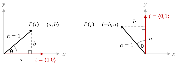
Since the length of a rotated vector does not change, we know the hypotenuse $h$ will always have a length of $1$ for basis vectors. That means $\sin(\theta)=\frac{b}{1}=b$ and $\cos(\theta)=\frac{a}{1}=a$ and we can express $b$ and $a$ in terms of $\theta$ as $b = \sin(\theta)$ and $a = \cos(\theta)$. \(\begin{aligned} F(i) &= \langle a,b \rangle = \langle\cos(\theta),\sin(\theta)\rangle \\ F(j) &= \langle -b,a \rangle = \langle -\sin(\theta),\cos(\theta)\rangle \end{aligned}\)

Since we know that $F(i)$ and $F(j)$ together determine the transformation matrix $A$, then we can express $A$ in terms of the angle of rotation $\theta$: \(\begin{aligned} F\left(\begin{bmatrix} x \\ y \end{bmatrix}\right) &= \begin{bmatrix} a & -b \\ b & a \end{bmatrix} \cdot \begin{bmatrix} x \\ y \end{bmatrix} = \begin{bmatrix} \cos(\theta) & -\sin(\theta) \\ \sin(\theta) & \cos(\theta) \end{bmatrix} \cdot \begin{bmatrix} x \\ y \end{bmatrix} \\ A &= \begin{bmatrix} \cos(\theta) & -\sin(\theta) \\ \sin(\theta) & \cos(\theta) \end{bmatrix}\end{aligned}\)

In 2D rotations, the angle $\theta$ revolves around a single point, but in 3D that point becomes a line extending perpendicular to the angle of rotation. For example, the $xy$-plane is perpendicular to the $z$-axis, so we can say that rotation in 2D space (the $xy$ plane) is the same as rotation around the $z$-axis in 3D space. The difference is that vectors in 3D space have three components and a third standard basis vector $k$ for the $z$ component is required: $i= \langle 1,0,0 \rangle$, $j= \langle 0,1,0 \rangle$, and $k= \langle 0,0,1 \rangle$.

$z$-Axis Rotation

When rotating around the $z$-axis, the $z$ coordinates do not change while the $x$ and $y$ coordinates change in the same way as 2D rotation. So the standard basis vector transformations are, \(\begin{aligned} F(i) &= \langle \cos(\theta), \sin(\theta), 0 \rangle \\ F(j) &= \langle -\sin(\theta), \cos(\theta), 0 \rangle \\ F(k) &= \langle 0, 0, 1 \rangle \end{aligned}\) And the transformation matrix is, \(A_z=\begin{bmatrix} \cos(\theta) & -\sin(\theta) & 0 \\ \sin(\theta) & \cos(\theta) & 0 \\ 0 & 0 & 1 \end{bmatrix}\)

$x$-Axis Rotation

When the axis of rotation is the $x$-axis, the standard basis vector $i$ becomes parallel to the axis of rotation, and perpendicular to the rotation plane. This means the $x$-components do not change in the same way that $z$-components do not change when we rotate around the $z$-axis. Graphically, we can represent this with a diagram in which the $i$ vector is perpendicular to the rotation plane and the $j$ vector extends to the right. Then the $k$ vector will point up according to the structure of the 3D coordinate axes. In this diagram, the vector components $a$ and $b$ represent sides of the right triangles on the $yz$ plane at $x=0$. Here we show the vectors in terms of $\langle y, z \rangle$ for simplicity since we know $x = 0$.

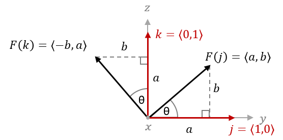
Now we can express $F(j)=\langle a,b \rangle$ and $F(k)=\langle -b,a \rangle$ in terms of $\theta$ to get our transformation matrix: \(A_x=\begin{bmatrix} 1 & 0 & 0 \\ 0 & a & -b \\ 0 & b & a \end{bmatrix} = \begin{bmatrix} 1 & 0 & 0 \\ 0 & \cos(\theta) & -\sin(\theta) \\ 0 & \sin(\theta) & \cos(\theta) \end{bmatrix}\)

$y$-Axis Rotation

Rotating around the $y$-axis is a little more complicated. To draw this diagram, it is important to remember the following points:

• The positive axis of rotation is perpendicular to the angle and points towards the viewer.
• The basis vector along the axis of rotation is ignored, and the other basis vectors are written in terms of the components on the plane of angle $\theta$.
• The first basis vector is drawn horizontally so that $\theta$ rotates counterclockwise from $\langle 1,0 \rangle$.
• And the second basis vector with value $\langle 0,1 \rangle$ is drawn vertically with its positive direction relative to the other two axes.

Following these rules, the diagram will have the $y$-axis pointing towards the viewer from the origin. We ignore the $j$ vector and write the components of the $i$ and $k$ vectors in terms of $x$ and $z$. Then the $x$-axis and its vector $i$ will point to the right while the $z$-axis and its vector $k$ will point down:

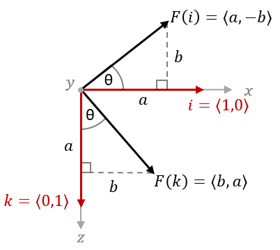
Now we can find our transformation matrix in terms of $\theta$ from $F(i)$ and $F(k)$ above: \(A_y=\begin{bmatrix} a & 0 & b \\ 0 & 1 & 0 \\ -b & 0 & a \end{bmatrix} = \begin{bmatrix} \cos(\theta) & 0 & \sin(\theta) \\ 0 & 1 & 0 \\ -\sin(\theta) & 0 & \cos(\theta) \end{bmatrix}\)

Finally, we can verify these matrices by considering what happens when $\theta =0$. At $\theta =0$, there should be no change to the coordinates since no rotation happens. In this case, plugging in $0$ for $\theta$ in each of these matrices will result in the identity matrix since $\cos(0)=1$ and $\sin(0)=0$. This is true for all three axes of rotation.

Translation

A translation simply changes the coordinate position of a vertex by a fixed value. Let’s use the constants $m$ and $n$ to show the change of $x$ and $y$ from translation $\langle m,n \rangle$: \(F\left(\begin{bmatrix} x \\ y \end{bmatrix}\right) = \begin{bmatrix} x+m \\ y+n \end{bmatrix}\)

Now, when we consider the nature of matrix multiplication, we see that a 2x2 matrix is not sufficient for adding constant values to each component. For example, consider a translation of $\langle 0,2 \rangle$ and try solving for $a$, $b$, $c$ and $d$: \(\begin{bmatrix} a & b \\ c & d \end{bmatrix} \cdot \begin{bmatrix} x \\ y \end{bmatrix} = \begin{bmatrix} a \cdot x+b \cdot y \\ c \cdot x+d \cdot y \end{bmatrix} = \begin{bmatrix} x \\ y+2 \end{bmatrix}\) From above, $a \cdot x+b \cdot y=x$ gives us the values $a=1$ and $b=0$. However, from $c \cdot x+d \cdot y=y+2$ we get $d=1$ and $c=2/x$ which is not constant. Even if we try to define our transformation matrix with $c=2/x$, then we would not be able to transform any coordinates where $x=0$ because $2/0$ is undefined. You might also recognize that $c=0$ would give us the identity matrix, which implies that $c$ must be some non-zero value.

Now if we try using a fixed value $c=2$ and apply the transformation to a square with points $(0,0)$, $(1,0)$, $(0,1)$ and $(1,1)$, we find another problem. \(F\left( (0,0) \right) = \begin{bmatrix} 1 & 0 \\ 2 & 1 \end{bmatrix} \cdot \begin{bmatrix} 0 \\ 0 \end{bmatrix} = (0,0) \\ F\left( (0,1) \right) = \begin{bmatrix} 1 & 0 \\ 2 & 1 \end{bmatrix} \cdot \begin{bmatrix} 0 \\ 1 \end{bmatrix} = (0,1) \\ F\left( (1,0) \right) = \begin{bmatrix} 1 & 0 \\ 2 & 1 \end{bmatrix} \cdot \begin{bmatrix} 1 \\ 0 \end{bmatrix} = (1,2) \\ F\left( (1,1) \right) = \begin{bmatrix} 1 & 0 \\ 2 & 1 \end{bmatrix} \cdot \begin{bmatrix} 1 \\ 1 \end{bmatrix} = (1,3) \\\)

We can see that the transformation only changes the $y$-coordinates for points where $x \neq 0$. This is called a shear translation and it warps the shape of the object. If we were to try this with a 3D object as well, then we would see only two of the three coordinates being translated. In other words, using a transformation matrix only applies the translation to a subset of the coordinate space.

A 2D vector can only be translated when it is a subset of a 3D system. So, we assume the point $(x,y)$ is on a plane in 3D space located at $z=1$ and then $(x,y)$ becomes $(x,y,1)$. Using these 3D coordinates, the transformation matrix is found simply: \(\begin{aligned} F\left(\begin{bmatrix} x \\ y \\ 1 \end{bmatrix}\right) &= \begin{bmatrix} x+m \\ y+n \\ 1 \end{bmatrix} = \begin{bmatrix} 1 & 0 & m \\ 0 & 1 & n \\ 0 & 0 & 1 \end{bmatrix} \cdot \begin{bmatrix} x \\ y \\ 1 \end{bmatrix} \\ A &= \begin{bmatrix} 1 & 0 & m \\ 0 & 1 & n \\ 0 & 0 & 1 \end{bmatrix} \end{aligned}\)

When we want to apply the 3D translation $\langle m,n,p \rangle$ in all three dimensions, we need to add a fourth dimension so that each point becomes $(x,y,z,1)$. Then the matrix calculation becomes: \(\begin{aligned} F\left(\begin{bmatrix} x \\ y \\ z \\ 1 \end{bmatrix}\right) &= \begin{bmatrix} x+m \\ y+n \\ z+p \\ 1 \end{bmatrix} = \begin{bmatrix} 1 & 0 & 0 & m \\ 0 & 1 & 0 & n \\ 0 & 0 & 1 & p \\ 0 & 0 & 0 & 1 \end{bmatrix} \cdot \begin{bmatrix} x \\ y \\ z \\ 1 \end{bmatrix} \\ A &= \begin{bmatrix} 1 & 0 & 0 & m \\ 0 & 1 & 0 & n \\ 0 & 0 & 1 & p \\ 0 & 0 & 0 & 1 \end{bmatrix} \end{aligned}\)

3D computer graphics always use 4D vectors and matrices to do 3D calculations. This system is called homogeneous coordinates. When we set the extra dimension equal to $1$, we get a useful correspondence between the 3D and 4D representatons of the point. That is, with 4D point $(x,y,z,w)$ we can divide $x$, $y$, and $z$ by $w$ to get the same point in 3D: \((x/w,y/w,z/w)=(x/1,y/1,z/1)=(x,y,z)\)

This is called perspective division and it provides some unique advantages for calculating the projections of a 3D scene (as we will see later in the section Perspective Projection).

If we are going to create a homogeneous coordinate system by adding an extra coordinate, then we should review the previous transformations with the new system applied. For 2D transformations, the function $F(\langle x,y \rangle)=\langle a \cdot x+b \cdot y,c \cdot x+d \cdot y \rangle$ becomes $F(\langle x,y,1 \rangle)=\langle a \cdot x+b \cdot y,c \cdot x+d \cdot y,1 \rangle$ and the matrix calculation is, \(\begin{bmatrix} a & b & 0 \\ c & d & 0 \\ 0 & 0 & 1 \end{bmatrix} \cdot \begin{bmatrix} x \\ y \\ 1 \end{bmatrix} = \begin{bmatrix} a \cdot x + b \cdot y \\ c \cdot x + d \cdot y \\ 1 \end{bmatrix} \\\)

Combine this matrix with the translation matrix and we get, \(\begin{bmatrix} a_{11} & a_{12} & m_1 \\ a_{21} & a_{22} & m_2 \\ 0 & 0 & 1 \end{bmatrix}\)

Here we can see the matrices for scaling and rotation combine nicely with the matrix for translation. The values $a_{11}$ to $a_{22}$ represent the scaling and rotation transformations while $m_1$ and $m_2$ are the translation values.

So the three transformations of scaling, rotation and translation (collectively called affine transformations) can be expressed together in a single matrix. If we further expand this out to 3D, that matrix will have an extra dimension as well: \(\begin{bmatrix} a_{11} & a_{12} & a_{13} & m_1 \\ a_{21} & a_{22} & a_{23} & m_2 \\ a_{31} & a_{32} & a_{33} & m_3 \\ 0 & 0 & 0 & 1 \end{bmatrix}\)

Projection

When rendering a 3D scene using OpenGL, we need to map coordinates of the viewable area to the coordinates of the clip space where all $x$, $y$, and $z$ coordinates are between the values of $+1.0$ and $-1.0$. Remember, in our previous programs we drew shapes with $x$ and $y$ coordinates in the range of $-1.0$ to $1.0$. That is the coordinate space of everything that OpenGL renders on screen. But when our scenes are defined in a much larger coordinate system, we need to map the vertices from the scene space to the clip space.

For this purpose, we need to calculate a volume of the world space that will be rendered on screen, called the viewing volume. There are different approaches to projecting coordinates from world space to screen space, but we will only cover the one that closely models human perspective in the real world.

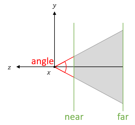
The View Frustum

We represent the viewable area using a shape called a frustum, which is basically a pyramid lying on its side with its tip cut off. It is centered around the the negative $z$-axis with its top represents the location of the viewer’s eye at the origin. The plane where the pyramids top is cut off represents the beginning of the viewable distance (often likened to the display screen) while the base of the pyramid is the end of the viewable distance. Everything inside the frustum will be rendered while all vertices outside the frustum are mostly ignored.

We can adjust this shape to make objects appear farther away or closer to the camera, and decide which objects to render based on their distance within a specified range. The values we use to adjust the frustum are the near distance, the far distance, the angle of view, and the aspect ratio.

The near distance and far distance are measured in units along the $z$-axis. The near distance (also called the near clipping distance) sets the limit for the closest viewable vertices. Likewise, the far distance (also called the far clipping distance) sets the limit for the farthest viewable vertices. When we choose not to render a point based on its location, this is called clipping.

The angle of view is the angle between the top and bottom planes of the frustum where they would intersect if they extended all the way to the origin.

From the point of view at the origin, the far distance plane appears to be the same size as the near distance plane. Since a rendered image is a 2D projection of a 3D scene, we must map all the points inside the frustum to the projection window. Imagine drawing a line from the origin to the point $P$. The point $Q$ where that line intersects with the projection window is the point that we render on screen.

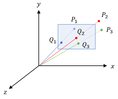
The size of the projection window determines the aspect ratio $r$ of the image. We define the aspect ratio with the width $w$ and height $h$ of the image as $r=w/h$.

Perspective Projection

The transformation that converts the coordinates of target vectors to coordinates of the clipping space is called perspective projection. In order to calculate this transformation, we need to find the matrix $A$ that will transform the target point $P$ from the world space to the point $Q$ in clipping space.

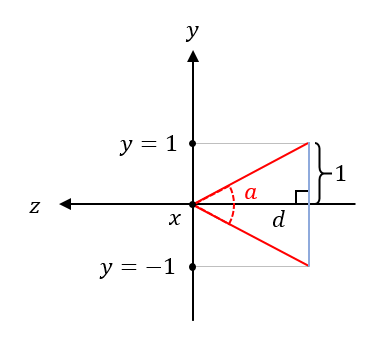
\[F(P)=A \cdot \begin{bmatrix} P_x \\ P_y \\ P_z \end{bmatrix} = \begin{bmatrix} Q_x \\ Q_y \\ Q_z \end{bmatrix} = Q\]

The bounds of the $x$-coordinates and $y$-coordinates in the clipping space are the same as the projection window. We define the projection window with the angle of view $a$ and $y$-coordinates between $-1$ and $1$. This will make it easier to use OpenGL which renders everything in a box with all coordinate values between $-1$ and $1$. Then, we know that the distance between the viewer and the projection window is $d=\frac{1}{\tan(a/2)}$.

Now, the right triangles formed by drawing a line through points $Q$ and point $P$ share the same angle. Since both triangles have the same $\tan(\theta)$, then we know $\frac{Q_y}{-d}=\frac{P_y}{P_z}$.

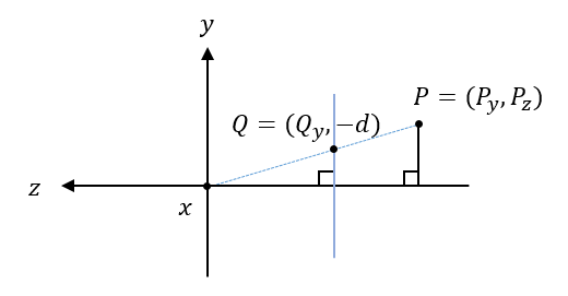
Solving for $Q_y$ then gives us $Q_y=\frac{d \cdot P_y}{-P_z}$. (Here we apply the negative to $P_z$ so that we can do a trick later.)

In terms of our transformation function, this equation tells us that, \(F(P)=A \cdot \begin{bmatrix} P_x \\ \\ P_y \\ \\ P_z \end{bmatrix} = \begin{bmatrix} Q_x \\ \\ \frac{d \cdot P_y}{-P_z} \\ \\ Q_z \end{bmatrix}\)

This does not look like a linear transformation yet because $Q_y$ depends on both $P_y$ and $-P_z$, but that is okay for now. Let’s look at the $x$-coordinates before coming back to this.

We find the $x$-coordinates in a similar way, looking at the right triangles that form with the line between $Q$ and $P$.

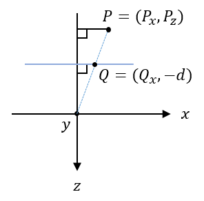
As before, we can find $Q_x$ with the equation $\frac{Q_x}{-d}=\frac{P_x}{P_z}$ to get $Q_x=\frac{d \cdot P_x}{-P_z}$. Now we also need to apply the aspect ratio $r$ to the $x$ values. Since our $y$ values are in the range $-1$ to $1$, then the $x$ values will be in the range $-r$ to $r$ which might not match the clipping space. In order to get the $x$ values into the range $-1$ to $1$ also, we divide by $r$. This effectively scales the range of $x$ values to the clipping space range. \(Q_x=\frac{d/r \cdot P_x}{-P_z}\)

And our transformation function is now: \(F(P)=A \cdot \begin{bmatrix} P_x \\ \\ P_y \\ \\ P_z \end{bmatrix} =\begin{bmatrix} \frac{d/r \cdot P_x}{-P_z} \\ \\ \frac{d \cdot P_y}{-P_z} \\ \\ Q_z \end{bmatrix}\)

Did you notice that both $Q_x$ and $Q_y$ have $-P_z$ in the denominator? This makes things easier when we work with homogeneous coordinates where our $(x,y,z)$ coordinates become $(x,y,z,w)$. In OpenGL, the GPU automatically calculates 3D vertices from 4D homogeneous coordinates with perspective division as below.

\[(x,y,z) = (x/w,y/w,z/w)\]

We can take advantage of perspective division to extract the $z$ component from the $x$ and $y$ components of $Q$. Specifically, $Q=(Q_x,Q_y,Q_z,Q_w)$ becomes $\left(\frac{Q_x}{Q_w},\frac{Q_y}{Q_w},\frac{Q_z}{Q_w}\right)$. Now if we set $Q_w=-P_z$, it solves our function very conveniently: \(F(P)=A \cdot \begin{bmatrix} P_x \\ \\ P_y \\ \\ P_z \\ \\ 1 \end{bmatrix} = \begin{bmatrix} \frac{d/r \cdot P_x}{-P_z} \\ \\ \frac{d \cdot P_y}{-P_z} \\ \\ \frac{Q_z}{-P_z} \\ \\ 1 \end{bmatrix} = \begin{bmatrix} d/r \cdot P_x \\ \\ d \cdot P_y \\ \\ Q_z \\ \\ -P_z \end{bmatrix}\)

Now we just need to understand $Q_z$ before we can assemble our complete transformation matrix $A$.

Remember that the view frustum lies parallel to the $z$-axis, so the values of the $z$-coordinates do not affect where the point is mapped onto the projection window. Instead, we only render points with $z$ values in between the near distance and far distance which define the visible space. With this in mind, we can express the calculation of $Q_z$ from $P$ with $0$ for the $x$ and $y$ components, and unknowns for the $z$ and $w$ components. That is, \(Q_z=A_z \cdot P = \begin{bmatrix} 0 & 0 & b & c \end{bmatrix} \cdot \begin{bmatrix} P_x \\ P_y \\ P_z \\ 1 \end{bmatrix}=b \cdot P_z + c\) Then apply perspective division from above to complete our transformation function: \(F(P_z)=\frac{Q_z}{-P_z}=\frac{A_z \cdot P}{-P_z}=\frac{b \cdot P_z+c}{-P_z}=-b-\frac{c}{P_z}\)

Now we just need to find values for $b$ and $c$. Since the frustum lies on the negative $z$-axis, we know that the nearest visible point will have $P_z=-n$ and the farthest will have $P_z=-f$. But the clipping space is bound by values $-1$ and $1$. In the clipping space of OpenGL, the $z$-axis is inverted, so the nearest $z$-coordinate of $P_z=-n$ will convert to $Q_z=-1$ and the farthest $z$-coordinate at $P_z=-f$ will convert to $Q_z=1$. This means that our expression from above gives:

\[-b-\frac{c}{-n}=-1 \quad \text{and} \quad -b-\frac{c}{-f}=1\]

Solving these two equations for the unknowns $b$ and $c$ then gives us

\[b=\frac{n+f}{n-f} \quad \textrm{and} \quad c=\frac{2 \cdot n \cdot f}{n-f}\]

Finally, let’s use all our equations from above and put together the components of the transformation matrix $A$, starting with the transformation vector for $x$: \(\begin{aligned} F(P_x)&=A_x \cdot \begin{bmatrix} P_x \\ P_y \\ P_z \\ 1 \end{bmatrix}=\frac{d}{r} \cdot P_x \\ A_x&=\begin{bmatrix} \frac{d}{r} & 0 & 0 & 0 \end{bmatrix} =\begin{bmatrix} \frac{1}{r \cdot \tan(a/2)} & 0 & 0 & 0 \end{bmatrix}\end{aligned}\)

Next is the transformation vector for $y$: \(\begin{aligned} F(P_y)&=A_y \cdot \begin{bmatrix} P_x \\ P_y \\ P_z \\ 1 \end{bmatrix}=d \cdot P_y \\ A_y&=\begin{bmatrix} 0 & d & 0 & 0 \end{bmatrix} =\begin{bmatrix} 0 & \frac{1}{\tan(a/2)} & 0 & 0 \end{bmatrix}\end{aligned}\)

Here is the $w$ transformation vector: \(\begin{aligned} F(P_w)&=A_w \cdot \begin{bmatrix} P_x \\ P_y \\ P_z \\ 1 \end{bmatrix}=-P_z \\ A_w&=\begin{bmatrix} 0 & 0 & -1 & 0 \end{bmatrix} \end{aligned}\)

And finally, the complete perspective projection transformation matrix includes all the components together: \(A=\begin{bmatrix} A_x \\ A_y \\ A_z \\ A_w \end{bmatrix} = \begin{bmatrix} \frac{1}{r \cdot \tan(a/2)} & 0 & 0 & 0 \\ 0 & \frac{1}{\tan(a/2)} & 0 & 0 \\ 0 & 0 & \frac{n+f}{n-f} & \frac{2 \cdot n \cdot f}{n-f} \\ 0 & 0 & -1 & 0 \end{bmatrix}\)

Here, $r$ is the aspect ratio, $a$ is the angle of view, $n$ is the near clipping distance, and $f$ is the far clipping distance. All of these will be configured by our applications.

Local Transformations

One important note about all these transformations so far is that they operate on vectors based at the origin. For example, if we have a rotation transformation $R$ of $45^{\circ}$ for an object with a set of points $P$ centered at $(0,0)$, then the transformation $R \cdot P$ rotates the object around its own center. However, if $P$ is centered on $(1,0)$ in the world space, then $R \cdot P$ applies the rotation to the object’s translation vector $\langle 1,0 \rangle$ and effectively rotates the object around the world origin.

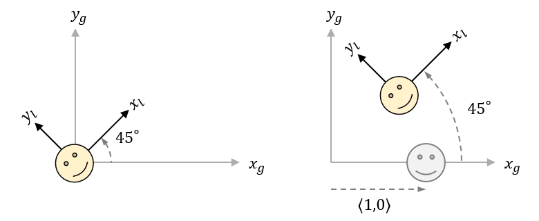
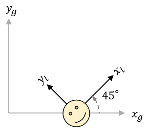
The picture on the left shows a rotation applied to object coordinates or local coordinates. Here, the rotation effectively transforms the object’s coordinate axes, which are shown as $x_l$ and $y_l$. The picture on the right shows the rotation applied to an object with its center at $(1,0)$ in the world coordinates or global coordinates defined by the $x_g$-axis and $y_g$-axis.

A local transformation is any transformation that applies relative to the local coordinates of an object. When an object’s local coordinates are the same as the world coordinates, any global transformation is also a local transformation on that object, as shown in the first image.

So how can we use our matrix multiplication method to perform a local transformation when the object is not at the global origin?

We must first understand that an object’s points are defined using local coordinates and OpenGL does not change these points when there is a transformation. Instead, it keeps a separate matrix, called a model matrix which is the cumulative product of all transformations on the object. Then, it calculates the world coordinates $P_g$ by multiplying the object’s local coordinates $P_l$ by the model matrix $M$.

\[P_g =M \cdot P_l\]

Naturally, when there are no transformations acting on the object, $M$ is the identity matrix.

\[P_g = M \cdot P_l = I \cdot P_l = P_l\]

If $M$ is the product of all transformations leading to the world coordinates of the object, then we know the inverse of $M$, denoted $M^{-1}$, will undo those transformations and give us the original object coordinates in local space. In other words, this converts the object’s coordinates from world space back to local coordinate space, like so:

\[P_l=M^{-1} \cdot P_g =M^{-1} \cdot M \cdot P_l\]

Once we have the local coordinates of the object, we can apply our rotation $R$ as a local transformation. Then, we move the object back to its previous world coordinates with transformation $M$ once more. Using matrix multiplication for this entire process, we can express the result $P_g’$ of applying local rotation $R$ to an object in world space as follows: \(\begin{aligned} P_g' &= M \cdot R \cdot M^{-1} \cdot P_g \\ &= M \cdot R \cdot M^{-1} \cdot M \cdot P_l \\ &= M \cdot R \cdot I \cdot P_l \\ &= M \cdot R \cdot P_l \end{aligned}\)

Remember that the nature of matrix multiplication implies the order of applying transormations goes from right to left. So for a local transformation, $R$ is applied before the model matrix: $P’ = M \cdot R \cdot P$. When we want to apply a global transformation, the transformation matrix $R$ is applied after the model matrix: $P’ = R \cdot M \cdot P$.

This conveniently applies to all previously discussed geometric transformations in addition to rotation.